使用 Q-Learning 解決 Blackjack

在本教學中，我們將探索並解決 Blackjack-v1 環境。

Blackjack 是最受歡迎的賭場紙牌遊戲之一，也因在某些條件下可以被擊敗而臭名昭著。此版本的遊戲使用無限牌組（我們抽牌時會放回牌組），因此在我們的模擬遊戲中，算牌不會是一種可行的策略。完整文件請見 https://gymnasium.dev.org.tw/environments/toy_text/blackjack

目標：為了獲勝，您的牌面總和應大於莊家，且不超過 21 點。

動作：代理可以在兩個動作之間選擇

• 停牌 (0)：玩家不再拿牌

• 叫牌 (1)：玩家將獲得另一張牌，但是玩家可能會超過 21 點而爆牌

方法：為了自行解決此環境，您可以選擇您最喜歡的離散 RL 演算法。提出的解決方案使用 Q-learning（一種無模型 RL 演算法）。

匯入與環境設定

# Author: Till Zemann
# License: MIT License

from __future__ import annotations

from collections import defaultdict

import matplotlib.pyplot as plt
import numpy as np
import seaborn as sns
from matplotlib.patches import Patch
from tqdm import tqdm

import gymnasium as gym


# Let's start by creating the blackjack environment.
# Note: We are going to follow the rules from Sutton & Barto.
# Other versions of the game can be found below for you to experiment.

env = gym.make("Blackjack-v1", sab=True)

# Other possible environment configurations are:

env = gym.make('Blackjack-v1', natural=True, sab=False)
# Whether to give an additional reward for starting with a natural blackjack, i.e. starting with an ace and ten (sum is 21).

env = gym.make('Blackjack-v1', natural=False, sab=False)
# Whether to follow the exact rules outlined in the book by Sutton and Barto. If `sab` is `True`, the keyword argument `natural` will be ignored.

觀察環境

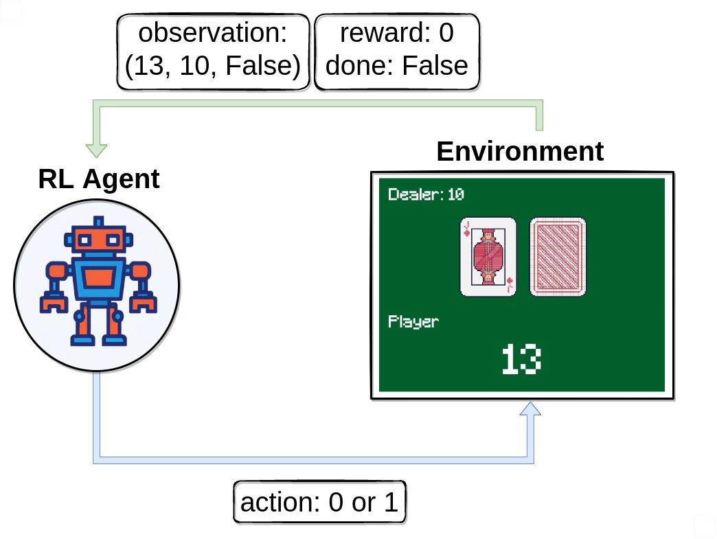
首先，我們呼叫 env.reset() 以開始一個回合。此函數將環境重置為起始位置，並傳回初始 observation。我們通常也會設定 done = False。此變數稍後將用於檢查遊戲是否終止（即玩家獲勝或失敗）。

# reset the environment to get the first observation
done = False
observation, info = env.reset()

# observation = (16, 9, False)

請注意，我們的觀察是一個由 3 個值組成的 3 元組

• 玩家目前的總和

• 莊家明牌的面值

• 布林值，表示玩家是否持有可用的 A 牌（如果 A 牌計為 11 點而不會爆牌，則為可用）

執行動作

在收到我們的第一個觀察結果後，我們只會使用 env.step(action) 函數與環境互動。此函數將動作作為輸入，並在環境中執行它。由於該動作會更改環境的狀態，因此它會傳回四個對我們有用的變數。這些是

• next_state：這是代理在採取動作後將收到的觀察結果。

• reward：這是代理在採取動作後將收到的獎勵。

• terminated：這是一個布林變數，指示環境是否已終止。

• truncated：這也是一個布林變數，指示回合是否因提前截斷而結束，即達到時間限制。

• info：這是一個字典，可能包含有關環境的其他資訊。

next_state、reward、terminated 和 truncated 變數是不言自明的，但 info 變數需要一些額外的解釋。此變數包含一個字典，其中可能包含有關環境的一些額外資訊，但在 Blackjack-v1 環境中，您可以忽略它。例如，在 Atari 環境中，info 字典有一個 ale.lives 鍵，告訴我們代理還剩下多少條命。如果代理有 0 條命，則回合結束。

請注意，在您的訓練迴圈中呼叫 env.render() 不是一個好主意，因為渲染會大大減慢訓練速度。而是嘗試建立一個額外的迴圈，在訓練後評估和展示代理。

# sample a random action from all valid actions
action = env.action_space.sample()
# action=1

# execute the action in our environment and receive infos from the environment
observation, reward, terminated, truncated, info = env.step(action)

# observation=(24, 10, False)
# reward=-1.0
# terminated=True
# truncated=False
# info={}

一旦 terminated = True 或 truncated=True，我們應該停止目前的回合，並使用 env.reset() 開始一個新的回合。如果您在不重置環境的情況下繼續執行動作，它仍然會回應，但輸出對於訓練沒有用處（如果代理學習了無效資料，甚至可能有害）。

建立代理

讓我們建立一個 Q-learning 代理 來解決 Blackjack-v1！我們需要一些函數來選擇動作並更新代理的動作值。為了確保代理探索環境，一種可能的解決方案是 epsilon-greedy 策略，我們以 epsilon 百分比選擇隨機動作，並以 1 - epsilon 百分比選擇貪婪動作（目前評估為最佳）。

class BlackjackAgent:
    def __init__(
        self,
        env,
        learning_rate: float,
        initial_epsilon: float,
        epsilon_decay: float,
        final_epsilon: float,
        discount_factor: float = 0.95,
    ):
        """Initialize a Reinforcement Learning agent with an empty dictionary
        of state-action values (q_values), a learning rate and an epsilon.

        Args:
            learning_rate: The learning rate
            initial_epsilon: The initial epsilon value
            epsilon_decay: The decay for epsilon
            final_epsilon: The final epsilon value
            discount_factor: The discount factor for computing the Q-value
        """
        self.q_values = defaultdict(lambda: np.zeros(env.action_space.n))

        self.lr = learning_rate
        self.discount_factor = discount_factor

        self.epsilon = initial_epsilon
        self.epsilon_decay = epsilon_decay
        self.final_epsilon = final_epsilon

        self.training_error = []

    def get_action(self, env, obs: tuple[int, int, bool]) -> int:
        """
        Returns the best action with probability (1 - epsilon)
        otherwise a random action with probability epsilon to ensure exploration.
        """
        # with probability epsilon return a random action to explore the environment
        if np.random.random() < self.epsilon:
            return env.action_space.sample()

        # with probability (1 - epsilon) act greedily (exploit)
        else:
            return int(np.argmax(self.q_values[obs]))

    def update(
        self,
        obs: tuple[int, int, bool],
        action: int,
        reward: float,
        terminated: bool,
        next_obs: tuple[int, int, bool],
    ):
        """Updates the Q-value of an action."""
        future_q_value = (not terminated) * np.max(self.q_values[next_obs])
        temporal_difference = (
            reward + self.discount_factor * future_q_value - self.q_values[obs][action]
        )

        self.q_values[obs][action] = (
            self.q_values[obs][action] + self.lr * temporal_difference
        )
        self.training_error.append(temporal_difference)

    def decay_epsilon(self):
        self.epsilon = max(self.final_epsilon, self.epsilon - self.epsilon_decay)

為了訓練代理，我們將讓代理一次玩一個回合（一個完整的遊戲稱為一個回合），然後在每個步驟後更新其 Q 值（遊戲中的單個動作稱為一個步驟）。

代理將必須體驗很多回合才能充分探索環境。

現在我們應該準備好建立訓練迴圈了。

# hyperparameters
learning_rate = 0.01
n_episodes = 100_000
start_epsilon = 1.0
epsilon_decay = start_epsilon / (n_episodes / 2)  # reduce the exploration over time
final_epsilon = 0.1

agent = BlackjackAgent(
    env=env,
    learning_rate=learning_rate,
    initial_epsilon=start_epsilon,
    epsilon_decay=epsilon_decay,
    final_epsilon=final_epsilon,
)

太棒了，讓我們開始訓練吧！

資訊：目前的超參數設定為快速訓練一個像樣的代理。如果您想收斂到最佳策略，請嘗試將 n_episodes 增加 10 倍，並降低 learning_rate（例如降至 0.001）。

env = gym.wrappers.RecordEpisodeStatistics(env, deque_size=n_episodes)
for episode in tqdm(range(n_episodes)):
    obs, info = env.reset()
    done = False

    # play one episode
    while not done:
        action = agent.get_action(env, obs)
        next_obs, reward, terminated, truncated, info = env.step(action)

        # update the agent
        agent.update(obs, action, reward, terminated, next_obs)

        # update if the environment is done and the current obs
        done = terminated or truncated
        obs = next_obs

    agent.decay_epsilon()

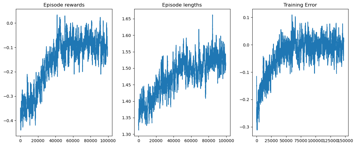
視覺化訓練

rolling_length = 500
fig, axs = plt.subplots(ncols=3, figsize=(12, 5))
axs[0].set_title("Episode rewards")
# compute and assign a rolling average of the data to provide a smoother graph
reward_moving_average = (
    np.convolve(
        np.array(env.return_queue).flatten(), np.ones(rolling_length), mode="valid"
    )
    / rolling_length
)
axs[0].plot(range(len(reward_moving_average)), reward_moving_average)
axs[1].set_title("Episode lengths")
length_moving_average = (
    np.convolve(
        np.array(env.length_queue).flatten(), np.ones(rolling_length), mode="same"
    )
    / rolling_length
)
axs[1].plot(range(len(length_moving_average)), length_moving_average)
axs[2].set_title("Training Error")
training_error_moving_average = (
    np.convolve(np.array(agent.training_error), np.ones(rolling_length), mode="same")
    / rolling_length
)
axs[2].plot(range(len(training_error_moving_average)), training_error_moving_average)
plt.tight_layout()
plt.show()

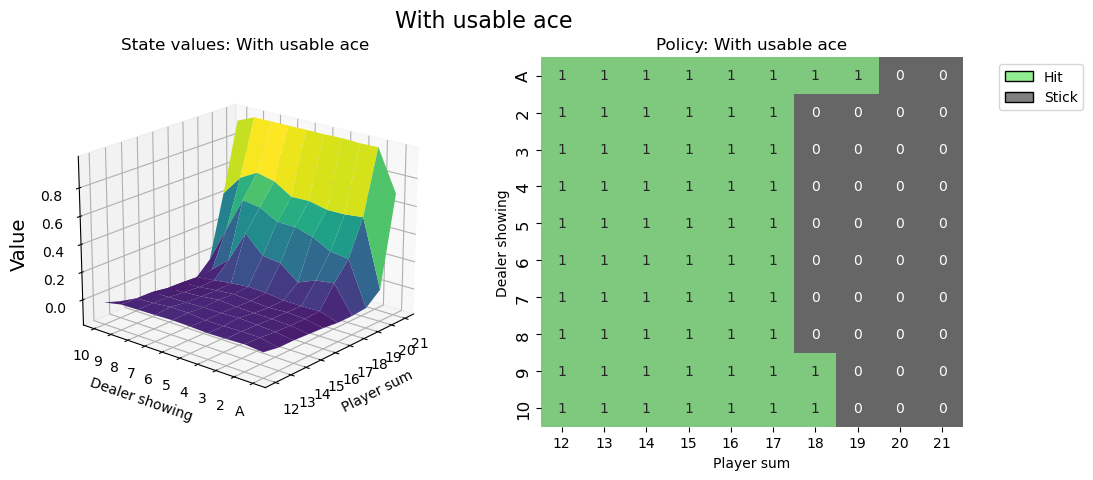
視覺化策略

def create_grids(agent, usable_ace=False):
    """Create value and policy grid given an agent."""
    # convert our state-action values to state values
    # and build a policy dictionary that maps observations to actions
    state_value = defaultdict(float)
    policy = defaultdict(int)
    for obs, action_values in agent.q_values.items():
        state_value[obs] = float(np.max(action_values))
        policy[obs] = int(np.argmax(action_values))

    player_count, dealer_count = np.meshgrid(
        # players count, dealers face-up card
        np.arange(12, 22),
        np.arange(1, 11),
    )

    # create the value grid for plotting
    value = np.apply_along_axis(
        lambda obs: state_value[(obs[0], obs[1], usable_ace)],
        axis=2,
        arr=np.dstack([player_count, dealer_count]),
    )
    value_grid = player_count, dealer_count, value

    # create the policy grid for plotting
    policy_grid = np.apply_along_axis(
        lambda obs: policy[(obs[0], obs[1], usable_ace)],
        axis=2,
        arr=np.dstack([player_count, dealer_count]),
    )
    return value_grid, policy_grid


def create_plots(value_grid, policy_grid, title: str):
    """Creates a plot using a value and policy grid."""
    # create a new figure with 2 subplots (left: state values, right: policy)
    player_count, dealer_count, value = value_grid
    fig = plt.figure(figsize=plt.figaspect(0.4))
    fig.suptitle(title, fontsize=16)

    # plot the state values
    ax1 = fig.add_subplot(1, 2, 1, projection="3d")
    ax1.plot_surface(
        player_count,
        dealer_count,
        value,
        rstride=1,
        cstride=1,
        cmap="viridis",
        edgecolor="none",
    )
    plt.xticks(range(12, 22), range(12, 22))
    plt.yticks(range(1, 11), ["A"] + list(range(2, 11)))
    ax1.set_title(f"State values: {title}")
    ax1.set_xlabel("Player sum")
    ax1.set_ylabel("Dealer showing")
    ax1.zaxis.set_rotate_label(False)
    ax1.set_zlabel("Value", fontsize=14, rotation=90)
    ax1.view_init(20, 220)

    # plot the policy
    fig.add_subplot(1, 2, 2)
    ax2 = sns.heatmap(policy_grid, linewidth=0, annot=True, cmap="Accent_r", cbar=False)
    ax2.set_title(f"Policy: {title}")
    ax2.set_xlabel("Player sum")
    ax2.set_ylabel("Dealer showing")
    ax2.set_xticklabels(range(12, 22))
    ax2.set_yticklabels(["A"] + list(range(2, 11)), fontsize=12)

    # add a legend
    legend_elements = [
        Patch(facecolor="lightgreen", edgecolor="black", label="Hit"),
        Patch(facecolor="grey", edgecolor="black", label="Stick"),
    ]
    ax2.legend(handles=legend_elements, bbox_to_anchor=(1.3, 1))
    return fig


# state values & policy with usable ace (ace counts as 11)
value_grid, policy_grid = create_grids(agent, usable_ace=True)
fig1 = create_plots(value_grid, policy_grid, title="With usable ace")
plt.show()

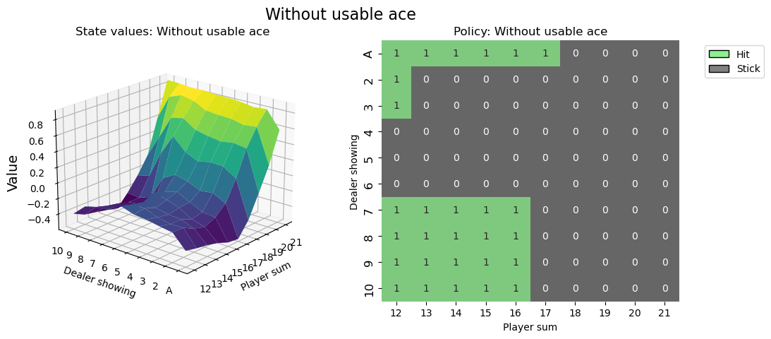
# state values & policy without usable ace (ace counts as 1)
value_grid, policy_grid = create_grids(agent, usable_ace=False)
fig2 = create_plots(value_grid, policy_grid, title="Without usable ace")
plt.show()

最好在腳本結尾呼叫 env.close()，以便關閉環境使用的任何資源。

認為您可以做得更好嗎？

# You can visualize the environment using the play function
# and try to win a few games.

希望本教學能幫助您掌握如何與 OpenAI-Gym 環境互動，並讓您踏上解決更多 RL 挑戰的旅程。

建議您自行解決此環境（基於專案的學習非常有效！）。您可以應用您最喜歡的離散 RL 演算法，或嘗試 Monte Carlo ES（在 Sutton & Barto 的 5.3 節中介紹）- 這樣您就可以將您的結果直接與書本進行比較。

祝您玩得開心！